How to Generate Stable Starting Values
Applying numerical algorithms and methods, the starting value of a variable is the value used for the first iteration. TESPy generates starting values for all variables automatically: known values propagate through the components, temperature levels are estimated and phase consistent enthalpies and saturation pressures are derived from them. The full process is described in the starting values section of the solver documentation. With this machinery most models converge without any help from the user.
With more complex models it can still happen, that the simulation does not converge from the automatically generated values. In that case, the strategy is to solve the model with a simpler but robust set of specifications first, for example directly imposing the saturation temperature levels of a heat pump cycle instead of terminal temperature differences. Since the solver starts from the previous solution, the actual specifications can then be imposed in a second solve: primary variables that hold a solved value do not need to be guessed anymore.
Here we provide a short tutorial for you to better understand, how this process could look like at the example of a subcritical heat pump with different working fluids.
Note
If the heat pump operates in trans- or supercritical range, some modifications have to be made on this setup. We plan to include respective examples here in the future.
You can download the full code of this example here:
starting_values.py
Topology of the heat pump
Following the first tutorial a slightly different topology for a heat pump with internal heat exchangers is considered instead of dumping the heat to the ambient. You can see the plant topology in the figure below.
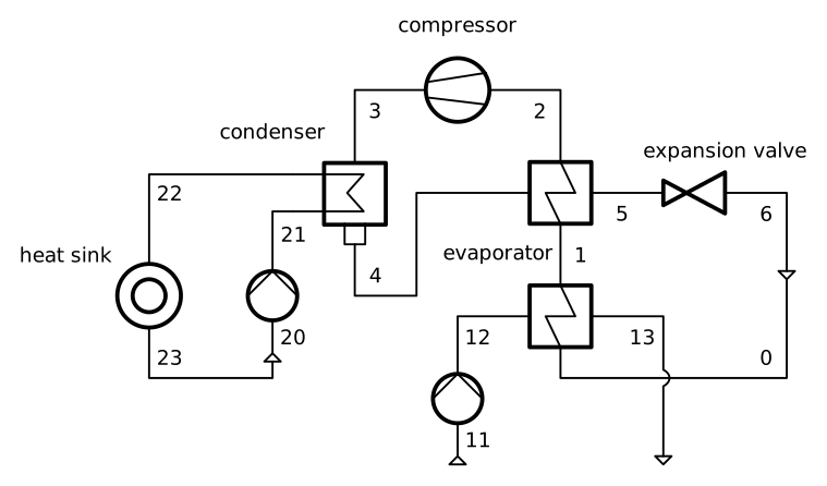
Figure: Topology of heat pump with internal heat exchanger

Figure: Topology of heat pump with internal heat exchanger
The system consists of a consumer system, a valve, an evaporator system, a compressor and additionally an internal heat exchanger. In order to simulate this heat pump, the TESPy model has to be built up. First, the network has to be initialized, and the refrigerants used have to be specified. This example shows how to make the heat pump model work with a variety of working fluids with water on both the heat source and heat sink side of the system.
Running into errors
As always, we start by importing the necessary TESPy classes.
from tespy.networks import Network

from tespy.components import (
    Condenser, Compressor, CycleCloser,  HeatExchanger,
    SimpleHeatExchanger, Pump, Sink, Source, Valve, PowerBus, PowerSource,
    HeatSink
    )

from tespy.connections import Connection, PowerConnection, HeatConnection
Then, we can build the network by defining components and connections. The working fluid will be set with the variable wf, “R290” is used in the first setup. This way, we will be able to change the working fluid in a flexible way.
Click to expand to code section
wf = "R290"

# network
nw = Network()
nw.units.set_defaults(
    temperature="degC", pressure="bar", enthalpy="kJ/kg", power="MW", heat="MW",
    pressure_difference="bar"
)

# components
cycle_closer = CycleCloser("Refrigerant Cycle Closer")

# heat source
heatsource_feedflow = Source("Heat Source Feed Flow")
heatsource_pump = Pump("Heat Source Recirculation Pump")
heatsource_evaporator = HeatExchanger("Heat Source Evaporator")
heatsource_backflow = Sink("Heat Source Back Flow")

# compression
compressor = Compressor("Compressor")

# heat sink
cons_pump = Pump("Heat Sink Recirculation Pump")
condenser = Condenser("Heat Sink Condenser")
cons_heatsink = SimpleHeatExchanger("Heat Consumer")
cons_cycle_closer = CycleCloser("Consumer Feed Flow")

# internal heat exchange
int_heatex = HeatExchanger("Internal Heat Exchanger")

# expansion
valve = Valve("Expansion Valve")

# connections
# main cycle
c0 = Connection(cycle_closer, "out1", heatsource_evaporator, "in2", label="0")
c1 = Connection(heatsource_evaporator, "out2", int_heatex, "in2", label="1")
c2 = Connection(int_heatex, "out2", compressor, "in1", label="2")
c3 = Connection(compressor, "out1", condenser, "in1", label="3")
c4 = Connection(condenser, "out1", int_heatex, "in1", label="4")
c5 = Connection(int_heatex, "out1", valve, "in1", label="5")
c6 = Connection(valve, "out1", cycle_closer, "in1", label="6")

nw.add_conns(c0, c1, c2, c3, c4, c5, c6)

# heat source
c11 = Connection(heatsource_feedflow, "out1", heatsource_pump, "in1", label="11")
c12 = Connection(heatsource_pump, "out1", heatsource_evaporator, "in1", label="12")
c13 = Connection(heatsource_evaporator, "out1", heatsource_backflow, "in1", label="13")

nw.add_conns(c11, c12, c13)

# heat sink
c21 = Connection(cons_cycle_closer, "out1", cons_pump, "in1", label="21")
c22 = Connection(cons_pump, "out1", condenser, "in2", label="22")
c23 = Connection(condenser, "out2", cons_heatsink, "in1", label="23")
c24 = Connection(cons_heatsink, "out1", cons_cycle_closer, "in1", label="24")

nw.add_conns(c21, c22, c23, c24)
After setting up the topology, the system’s parameters should be set in the following way:
Heat sink temperature levels (T at 23 and 24)
Heat source temperature levels (T at 11 and 13)
Degree of overheating after the internal heat exchanger (td_dew at 2)
Pinch point temperature difference at the evaporator (ttd_l) to derive evaporation pressure
Temperature difference at the condenser (ttd_u) to derive condensation pressure
Saturated gaseous state of the working fluid (x=1) after leaving the evaporator
Efficiencies of pumps and the compressor (eta_s)
Pressure losses in all heat exchangers (pr1, pr2, pr)
Consumer heat demand (Q)
Click to expand to code section
# parametrization connections
# set feedflow and backflow temperature of heat source and consumer
T_hs_bf = 10
T_hs_ff = 15
T_cons_bf = 50
T_cons_ff = 70

# consumer cycle
c23.set_attr(T=T_cons_ff, p=10, fluid={"water": 1})
c24.set_attr(T=T_cons_bf)

# heat source cycle
c11.set_attr(T=T_hs_ff, p=1, fluid={"water": 1})
c13.set_attr(T=T_hs_bf, p=1)

# evaporation to fully saturated gas
c1.set_attr(x=1, fluid={wf: 1})
# degree of overheating after internal heat exchanger (evaporation side)
c2.set_attr(td_dew=10)

# parametrization components
# isentropic efficiency
cons_pump.set_attr(eta_s=0.8)
heatsource_pump.set_attr(eta_s=0.8)
compressor.set_attr(eta_s=0.85)

# pressure ratios
condenser.set_attr(pr1=0.98, pr2=0.98)
heatsource_evaporator.set_attr(pr1=0.98, pr2=0.98)
cons_heatsink.set_attr(pr=0.99)
int_heatex.set_attr(pr1=0.98, pr2=0.98)

# temperature differences
heatsource_evaporator.set_attr(ttd_l=5)
condenser.set_attr(ttd_u=5)

# consumer heat demand
cons_heatsink.set_attr(Q=-1)

try:
    nw.solve("design")
except ValueError as e:
    print(e)
The system should be well defined with the parameter settings, however the solver does not find a solution from the automatically generated starting values. It isolates the part of the problem it fails on and reports it:
Error
Block 5 did not converge, solving the remaining 2 blocks simultaneously.
  Cause: no acceptance within the iteration budget of 50 iterations,
  the last scaled residual is 1.86e-02
  Equations: Compressor.eta_s,
  Heat Sink Condenser.energy_balance_constraints,
  Heat Source Evaporator.ttd_l,
  Internal Heat Exchanger.energy_balance_constraints, 1.x, 2.td_dew
  Variables: h0, h1, h4, m6, h7, p11
The remaining system did not converge either, restarting with the
simultaneous solution of the full system from its initial state.
The solver does not seem to make any progress, aborting calculation.
Scaled residual value is 1.86e-02 (1: x)
Possible reasons include:
 - fluid properties moving outside the valid range of the property
   database (consider adjusting p_range or h_range),
 - an impossible constraint that can never be satisfied
 - bad starting values causing the Newton solver to diverge.
Use nw.print_residuals() to identify which equations have the largest
residuals.
The messages already narrow the failure down: the equation system was
decomposed into blocks and every block
solved fine except one. The group of six coupled equations determining the
evaporation side of the cycle failed. Neither solving the remaining blocks in
one coupled system nor restarting with the full system finds the solution, so
the calculation ends with nw.status == 2.
Tip
To investigate such a failure interactively, the solver can pause at the failing block instead of escalating:
nw.solve("design", pause_on_block_failure=True)
nw.print_block_states(block=5, at="failure")
nw.print_block_jacobian(block=5)
The state tables show the fluid states the newton algorithm diverged to,
the variable values of the failed block can be modified and the solution
process continued with nw.solve_continue(). The section on
interacting with the solver describes the
workflow in detail.
Fixing the errors
All equations of the failed block are tied to the pressure and enthalpy levels of the evaporation side of the cycle, so this is where better starting values are required. To provide them, it is recommended to fix the saturation levels of the cycle directly instead of the temperature differences in a first calculation. In this example, the fixed points can be identified with the help of the logph diagram which you can see in the figure below.
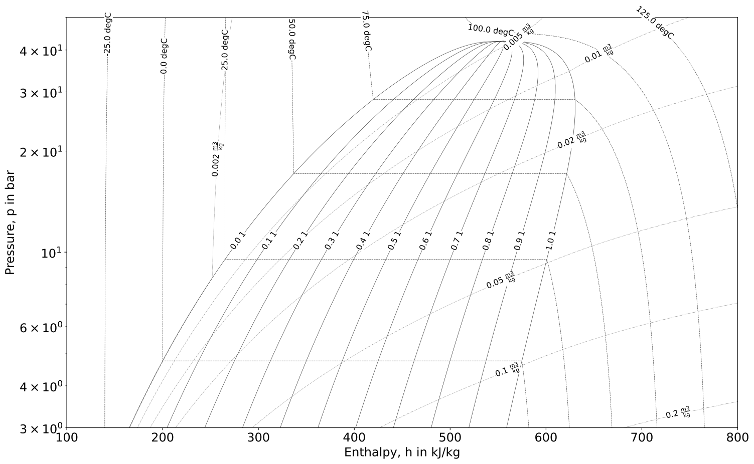
Figure: Logph diagram of propane
Figure: Logph diagram of propane
A rough estimation of the evaporation and condensation temperature can be
obtained from the temperature levels of the heat source and the heat sink.
Evaporation takes place a few Kelvin below the heat source backflow
temperature, condensation a few Kelvin above the consumer feed flow
temperature. These estimates can be imposed directly through the dew line
temperature T_dew at the evaporator outlet and the bubble line
temperature T_bubble at the condenser outlet. Each of them fixes the
pressure of its saturation state.
The terminal temperature differences are unset and the saturation temperatures are set instead.
# evaporation point
c1.set_attr(T_dew=T_hs_bf - 5)
heatsource_evaporator.set_attr(ttd_l=None)

# condensation point
c4.set_attr(T_bubble=T_cons_ff + 5)
condenser.set_attr(ttd_u=None)

# solve the network again
nw.solve("design")
The model was solved successfully and has stored the starting values for any follow-up. Therefore, we can undo our recent changes and restart the simulation. For example, the COP is then calculated.
# evaporation point
c1.set_attr(T_dew=None)
heatsource_evaporator.set_attr(ttd_l=5)

# condensation point
c4.set_attr(T_bubble=None)
condenser.set_attr(ttd_u=5)

# internal heat exchanger superheating
c2.set_attr(td_dew=5)

# solve the network again
nw.solve("design")

# calculate the COP
cop = abs(
    cons_heatsink.Q.val
    / (cons_pump.P.val + heatsource_pump.P.val + compressor.P.val)
)
print(cop)
Expand fix to any working fluids
Finally, using this strategy, it is possible to build a generic function, building a network, that works with a variety of working fluids.
Click to expand to code section
def generate_network_with_starting_values(wf):
    # network
    nw = Network(iterinfo=False)
    nw.units.set_defaults(
        temperature="degC", pressure="bar", enthalpy="kJ/kg", power="MW",
        heat="MW", pressure_difference="bar"
    )

    # components
    cycle_closer = CycleCloser("Refrigerant Cycle Closer")

    # heat source
    heatsource_feedflow = Source("Heat Source Feed Flow")
    heatsource_pump = Pump("Heat Source Recirculation Pump")
    heatsource_evaporator = HeatExchanger("Heat Source Evaporator")
    heatsource_backflow = Sink("Heat Source Back Flow")

    # compression
    compressor = Compressor("Compressor")

    # heat sink
    cons_pump = Pump("Heat Sink Recirculation Pump")
    condenser = Condenser("Heat Sink Condenser")
    cons_heatsink = SimpleHeatExchanger("Heat Consumer")
    cons_cycle_closer = CycleCloser("Consumer Feed Flow")

    # internal heat exchange
    int_heatex = HeatExchanger("Internal Heat Exchanger")

    # expansion
    valve = Valve("Expansion Valve")

    # connections
    # main cycle
    c0 = Connection(cycle_closer, "out1", heatsource_evaporator, "in2", label="0")
    c1 = Connection(heatsource_evaporator, "out2", int_heatex, "in2", label="1")
    c2 = Connection(int_heatex, "out2", compressor, "in1", label="2")
    c3 = Connection(compressor, "out1", condenser, "in1", label="3")
    c4 = Connection(condenser, "out1", int_heatex, "in1", label="4")
    c5 = Connection(int_heatex, "out1", valve, "in1", label="5")
    c6 = Connection(valve, "out1", cycle_closer, "in1", label="6")

    nw.add_conns(c0, c1, c2, c3, c4, c5, c6)

    # heat source
    c11 = Connection(heatsource_feedflow, "out1", heatsource_pump, "in1", label="11")
    c12 = Connection(heatsource_pump, "out1", heatsource_evaporator, "in1", label="12")
    c13 = Connection(heatsource_evaporator, "out1", heatsource_backflow, "in1", label="13")

    nw.add_conns(c11, c12, c13)

    # heat sink
    c21 = Connection(cons_cycle_closer, "out1", cons_pump, "in1", label="20")
    c22 = Connection(cons_pump, "out1", condenser, "in2", label="21")
    c23 = Connection(condenser, "out2", cons_heatsink, "in1", label="22")
    c24 = Connection(cons_heatsink, "out1", cons_cycle_closer, "in1", label="23")

    nw.add_conns(c21, c22, c23, c24)

    # set feedflow and backflow temperature of heat source and consumer
    T_hs_bf = 10
    T_hs_ff = 15
    T_cons_bf = 50
    T_cons_ff = 70

    # consumer cycle
    c23.set_attr(T=T_cons_ff, p=10, fluid={"water": 1})
    c24.set_attr(T=T_cons_bf)

    # heat source cycle
    c11.set_attr(T=T_hs_ff, p=1, fluid={"water": 1})
    c13.set_attr(T=T_hs_bf, p=1)

    # evaporation to fully saturated gas
    c1.set_attr(x=1, fluid={wf: 1})

    # parametrization components
    # isentropic efficiency
    cons_pump.set_attr(eta_s=0.8)
    heatsource_pump.set_attr(eta_s=0.8)
    compressor.set_attr(eta_s=0.85)

    # pressure ratios
    condenser.set_attr(pr1=0.98, pr2=0.98)
    heatsource_evaporator.set_attr(pr1=0.98, pr2=0.98)
    cons_heatsink.set_attr(pr=0.99)
    int_heatex.set_attr(pr1=0.98, pr2=0.98)

    # evaporation point
    c1.set_attr(T_dew=T_hs_bf - 5)

    # condensation point
    c4.set_attr(T_bubble=T_cons_ff + 5)

    # internal heat exchanger superheating
    c2.set_attr(td_dew=5)

    # consumer heat demand
    cons_heatsink.set_attr(Q=-1.0)

    grid = PowerSource("grid")
    electricity = PowerBus("electricity distribution", num_in=1, num_out=3)
    heat = HeatSink("heat production")
    e1 = PowerConnection(grid, "power", electricity, "power_in1", label="e1")
    e2 = PowerConnection(electricity, "power_out1", compressor, "power", label="e2")
    e3 = PowerConnection(electricity, "power_out2", cons_pump, "power", label="e3")
    e4 = PowerConnection(electricity, "power_out3", heatsource_pump, "power", label="e4")

    h1 = HeatConnection(cons_heatsink, "heat", heat, "heat", label="h1")
    nw.add_conns(e1, e2, e3, e4, h1)

    nw.solve("design")

    # evaporation point
    c1.set_attr(T_dew=None)
    heatsource_evaporator.set_attr(ttd_l=5)

    # condensation point
    c4.set_attr(T_bubble=None)
    condenser.set_attr(ttd_u=5)

    # solve the network again
    nw.solve("design")
    nw.assert_convergence()

    return nw
We can run that function for different working fluids and plot the results:
import matplotlib.pyplot as plt
import pandas as pd


# make text reasonably sized
plt.rc("font", **{"size": 18})

cop = pd.DataFrame(columns=["COP"])

for wf in ["NH3", "R22", "R134a", "R152a", "R290", "R718"]:
    nw = generate_network_with_starting_values(wf)

    power = nw.get_conn("e1").E.val
    heat = nw.get_conn("h1").E.val
    cop.loc[wf] = heat / power

fig, ax = plt.subplots(1, figsize=(16, 8))

cop.plot.bar(ax=ax, legend=False)

ax.set_axisbelow(True)
ax.yaxis.grid(linestyle="dashed")
ax.set_xlabel("Name of working fluid")
ax.set_ylabel("Coefficicent of performance")
plt.tight_layout()

fig.savefig("COP_by_wf.svg")
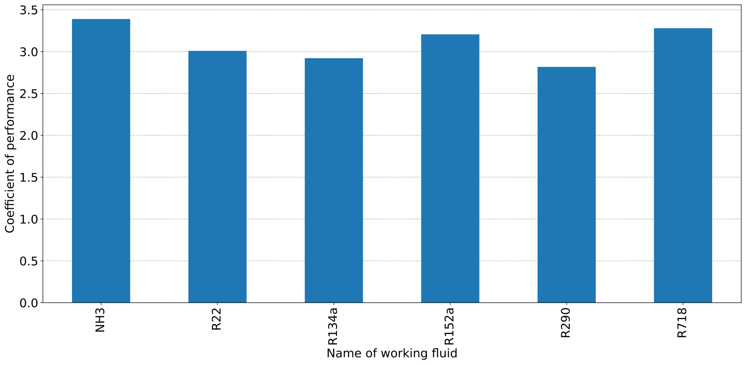
Figure: Analysis of the COP using different working fluids

Figure: Analysis of the COP using different working fluids