CO2 refrigeration system

This notebook models a CO2 transcritical booster refrigeration system of the kind used in supermarkets. The model is built with TESPy and CoolProp for the R744 (CO2) property data.

The booster-cycle topology, component set, and boundary conditions used here (evaporator pressures and cooling loads, compressor isentropic efficiencies, gas cooler pressure and outlet temperature, receiver pressure) are taken from:

Francesco D”Ettorre, Christian Heerup, “Chapter 5 - Modelling of a commercial refrigeration system in Python”, Case Studies in Energy Systems, Elsevier, 2026, Pages 163-189, ISBN 9780443238635, https://doi.org/10.1016/B978-0-443-23863-5.00010-5.

The model is implemented as a subclass of tespy”s ModelTemplate class, which provides the parameter handling, solving with automatic recovery, fluid property diagram plotting, sensitivity analysis and optimization plumbing. On top of the case study itself, the notebook shows how to

• run the subcritical baseline case and inspect performance indicators,

• plot cycle and heat exchanger TQ diagrams,

• switch to transcritical operation at high ambient temperature,

• run a sensitivity analysis on the gas cooler pressure to visualize the COP trade-off in transcritical operation, and

• find the COP-optimal combination of gas cooler and receiver pressure with pymoo.

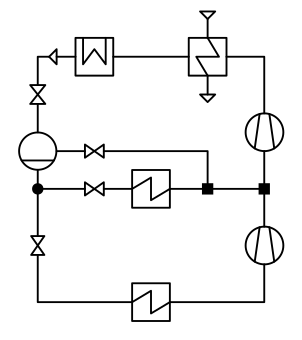
The flowsheet of the CO2 system is shown below.

Imports

Everything model related comes from tespy: the components and connections to build the network and the ModelTemplate base class from tespy.models. FluidPropertyDiagram from fluprodia draws the background isolines of the log(p)-h diagrams and PSO (particle swarm optimization) from pymoo is the optimization algorithm used later.

import os

import matplotlib.pyplot as plt
import numpy as np
import pandas as pd
from fluprodia import FluidPropertyDiagram
from pymoo.algorithms.soo.nonconvex.pso import PSO

from tespy.components import (
    Sink, Source, SimpleHeatExchanger, CycleCloser, Valve, Compressor,
    DropletSeparator, Merge, Splitter, SectionedHeatExchanger
)
from tespy.connections import Connection
from tespy.models import ModelTemplate
from tespy.networks import Network

The CO2BoosterModel class

ModelTemplate requires the implementation of a small number of methods:

• _create_network builds the topology, applies initial boundary conditions and solves the model once, so that a stable solution is available. The base class falls back to that solution automatically whenever a later solve corrupts the model.

• _parameter_lookup maps flat, human readable parameter names to their location in the network, e.g. ["Connections", "c10", "p"]. These names are the single interface used by set_parameters, get_parameter, the sensitivity analysis and the optimizer.

• solve_model is the entry point the optimizer calls. In this example it simply runs a design simulation.

Besides the settable parameters, the lookup also contains read-only indicators using the {"get": callable} form. The coefficient of performance relates the two cooling loads to the total compression power

\[\mathrm{COP} = \frac{\dot{Q}_\mathrm{evap,LT} + \dot{Q}_\mathrm{evap,MT}}{P_\mathrm{comp,LT} + P_\mathrm{comp,MT}}\]

and the flash gas fraction is the share of vapor bypassed from the receiver in the total high pressure valve mass flow

\[x_\mathrm{flash} = \frac{\dot{m}_\mathrm{c16}}{\dot{m}_\mathrm{c3}}.\]

Both getters return nan if the last solve did not converge. The optimizer uses this information to penalize such objectives automatically, so failed evaluations are discarded.

Finally, _get_diagram overrides the diagram setup of the base class. The default isolines only cover subcritical states, but the CO2 cycle crosses the critical point, so temperature isolines up to 150 °C and vapor quality isolines are calculated instead.

class CO2BoosterModel(ModelTemplate):

    def _parameter_lookup(self) -> dict:
        return {
            "lt_evaporator_load_kW": ["Components", "lt-evaporator", "Q"],
            "mt_evaporator_load_kW": ["Components", "mt-evaporator", "Q"],
            "lt_compressor_isentropic_eff": ["Components", "lt-compressor", "eta_s"],
            "mt_compressor_isentropic_eff": ["Components", "mt-compressor", "eta_s"],
            "lt_evaporator_pressure_bar": ["Connections", "c6", "p"],
            "mt_evaporator_pressure_bar": ["Connections", "c13", "p"],
            "receiver_pressure_bar": ["Connections", "c3", "p"],
            "gas_cooler_pressure_bar": ["Connections", "c10", "p"],
            "gas_cooler_outlet_temperature_C": ["Connections", "c1", "T"],
            "gas_cooler_discharge_kW": ["Components", "gas-cooler", "Q"],
            "hrhx_water_inlet_temperature_C": ["Connections", "c11", "T"],
            "mt_compressor_power_kW": ["Components", "mt-compressor", "P"],
            "lt_compressor_power_kW": ["Components", "lt-compressor", "P"],
            "hrhx_heat_kW": ["Components", "heat-recovery-heat-exchanger", "Q"],
            "discharge_temperature_C": ["Connections", "c10", "T"],
            "COP": {"get": self._calc_cop},
            "total_compressor_power_kW": {"get": self._calc_total_power},
            "flash_gas_fraction": {"get": self._calc_flash_gas_fraction},
        }

    def _calc_cop(self) -> float:
        if not self._solved:
            return np.nan
        Q_total = (
            self.get_parameter("lt_evaporator_load_kW")
            + self.get_parameter("mt_evaporator_load_kW")
            - self.get_parameter("hrhx_heat_kW")
        )
        return Q_total / self._calc_total_power()

    def _calc_total_power(self) -> float:
        if not self._solved:
            return np.nan
        return (
            self.get_parameter("lt_compressor_power_kW")
            + self.get_parameter("mt_compressor_power_kW")
        )

    def _calc_flash_gas_fraction(self) -> float:
        if not self._solved:
            return np.nan
        return self.nw.get_conn("c16").m.val / self.nw.get_conn("c3").m.val

    def solve_model(self, **kWargs) -> None:
        self.solve_model_design(**kWargs)

    def _get_diagram(self, fluid_name):
        if fluid_name not in self._diagram_cache:
            diagram = FluidPropertyDiagram(fluid_name)
            diagram.set_unit_system(self.nw.units)
            diagram.set_isolines(
                T=np.arange(-50, 160, 10),
                p=np.array([]),
                h=np.array([]),
                s=np.array([]),
                vol=np.array([]),
                Q=np.linspace(0, 1, 11)
            )
            diagram.calc_isolines()
            self._diagram_cache[fluid_name] = diagram
        return self._diagram_cache[fluid_name]

    def _create_network(self) -> None:
        self.nw = Network(iterinfo=False)
        self.nw.units.set_defaults(
            temperature="°C", pressure="bar", pressure_difference="bar",
            enthalpy="kJ/kg", heat="kW", power="kW"
        )

        # === System components =========================================
        gas_cooler = SimpleHeatExchanger("gas-cooler")
        cc = CycleCloser("cc")
        hp_valve = Valve("high-pressure-valve")
        bp_valve = Valve("by-pass-valve")
        mt_exp_valve = Valve("mt-exp-valve")
        lt_exp_valve = Valve("lt-exp-valve")
        mt_evap = SimpleHeatExchanger("mt-evaporator")
        lt_evap = SimpleHeatExchanger("lt-evaporator")
        mt_comp = Compressor("mt-compressor")
        lt_comp = Compressor("lt-compressor")
        merge1 = Merge("mt-evaporator-outlet")
        merge2 = Merge("mt-compressor-suction")
        split = Splitter("receiver-liq-outlet")
        receiver = DropletSeparator("receiver")
        hrhx = SectionedHeatExchanger("heat-recovery-heat-exchanger")
        water_inlet = Source("water-inlet")
        water_outlet = Sink("water-outlet")

        # === Connections ===============================================
        w1 = Connection(water_inlet, "out1", hrhx, "in2", "w1")
        w2 = Connection(hrhx, "out2", water_outlet, "in1", "w2")

        c1 = Connection(gas_cooler, "out1", cc, "in1", "c1")
        c2 = Connection(cc, "out1", hp_valve, "in1", "c2")
        c3 = Connection(hp_valve, "out1", receiver, "in1", "c3")
        c4 = Connection(receiver, "out1", split, "in1", "c4")
        c5 = Connection(split, "out1", lt_exp_valve, "in1", "c5")
        c6 = Connection(lt_exp_valve, "out1", lt_evap, "in1", "c6")
        c7 = Connection(lt_evap, "out1", lt_comp, "in1", "c7")
        c8 = Connection(lt_comp, "out1", merge2, "in1", "c8")
        c9 = Connection(merge2, "out1", mt_comp, "in1", "c9")
        c10 = Connection(mt_comp, "out1", hrhx, "in1", "c10")
        c11 = Connection(hrhx, "out1", gas_cooler, "in1", "c11")
        c12 = Connection(split, "out2", mt_exp_valve, "in1", "c12")
        c13 = Connection(mt_exp_valve, "out1", mt_evap, "in1", "c13")
        c14 = Connection(mt_evap, "out1", merge1, "in1", "c14")
        c15 = Connection(merge1, "out1", merge2, "in2", "c15")
        c16 = Connection(receiver, "out2", bp_valve, "in1", "c16")
        c17 = Connection(bp_valve, "out1", merge1, "in2", "c17")

        self.nw.add_conns(
            c1, c2, c3, c4, c5, c6, c7, c8, c9, c10, c11, c12, c13, c14,
            c15, c16, c17, w1, w2
        )

        # === Component parametrisation ==================================
        gas_cooler.set_attr(dp=0)
        hrhx.set_attr(dp1=0, dp2=0, td_pinch=5)
        mt_comp.set_attr(eta_s=.8)
        lt_comp.set_attr(eta_s=.85)
        mt_evap.set_attr(pr=1, Q=75)
        lt_evap.set_attr(pr=1, Q=25)

        c1.set_attr(T=15, fluid={"R744": 1})
        c3.set_attr(p=32)
        c6.set_attr(p=13)
        c13.set_attr(p=26)
        c10.set_attr(p=57.3)
        c7.set_attr(td_dew=10)
        c14.set_attr(td_dew=10)

        w1.set_attr(T=30, p=3, fluid={"water": 1})
        w2.set_attr(T=55)

        # === Solve ======================================================
        self.nw.solve("design")

        self._solved = self.nw.status == 0
        self._stable_solution = self.nw.save(as_dict=True)

Case Study 1 - subcritical baseline

The first run uses the operating conditions of Case Study 1 from the book chapter:

Parameter	Value
LT evaporator pressure	13 bar (≈ -33 °C)
MT evaporator pressure	26 bar (≈ -10 °C)
Receiver pressure	32 bar
Gas cooler pressure	57.3 bar
Gas cooler outlet temperature	15 °C (5 °C subcooling)
LT cooling load	25 kW
MT cooling load	75 kW
LT compressor isentropic efficiency	0.85
MT compressor isentropic efficiency	0.80

These match the defaults hardcoded in _create_network, so passing them through solve_model here is intended to show how values enter the model through the flat parameter interface.

After the solve, get_results collects the performance indicators defined in the lookup. Note that the heat recovery duty is negative by TESPy sign convention.

case_study_1 = {
    "lt_evaporator_pressure_bar": 13,
    "mt_evaporator_pressure_bar": 26,
    "receiver_pressure_bar": 32,
    "gas_cooler_pressure_bar": 57.3,
    "gas_cooler_outlet_temperature_C": 15,
    "lt_evaporator_load_kW": 25,
    "mt_evaporator_load_kW": 75,
    "lt_compressor_isentropic_eff": 0.85,
    "mt_compressor_isentropic_eff": 0.80,
}

indicators = [
    "COP", "total_compressor_power_kW", "hrhx_heat_kW", "flash_gas_fraction",
    "discharge_temperature_C", "gas_cooler_pressure_bar", "receiver_pressure_bar",
    "gas_cooler_discharge_kW"
]

model = CO2BoosterModel()
model.solve_model(**case_study_1)

records = {}
records["case study 1"] = model.get_results(indicators)
pd.Series(records["case study 1"], name="case study 1")

COP                            4.942799
total_compressor_power_kW     25.167855
hrhx_heat_kW                 -24.399647
flash_gas_fraction             0.189657
discharge_temperature_C       68.554425
gas_cooler_pressure_bar       57.300000
receiver_pressure_bar         32.000000
gas_cooler_discharge_kW     -100.768208
Name: case study 1, dtype: float64

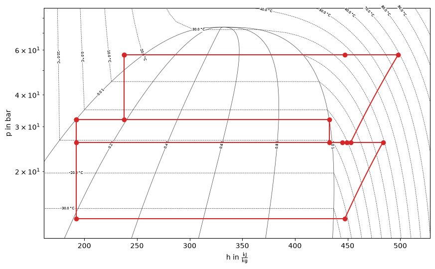
The log(p)-h diagram can automatically be generated with plot_logph_diagram_matplotlib. It extracts all process lines of the cycle starting from connection c1 and the diagram limits are derived from the actual state points. With the gas cooler outlet at 15 °C and 57.3 bar, the heat rejection ends below the critical point inside the subcooled liquid region.

fig, ax = model.plot_logph_diagram_matplotlib("c1")

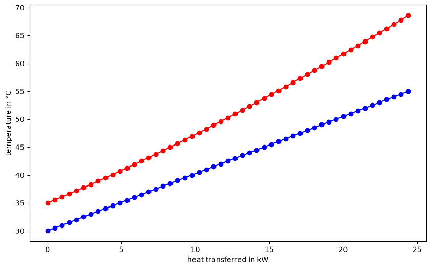
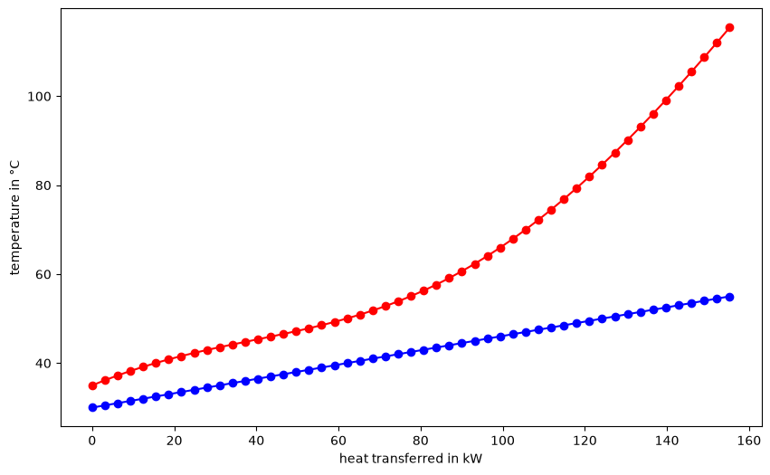
We can also generate TQ diagrams for heat exchangers that have both a hot and a cold side. This is the case for the heat recovery heat exchanger.

fig, ax = model.plot_QT_diagram_matplotlib("heat-recovery-heat-exchanger")

Transcritical operation at high ambient temperature

CO2 has a critical temperature of only 31 °C. On a hot day the gas cooler can no longer condense the refrigerant at subcritical pressure. For example, we assume an outlet temperature of 35 °C. Then the heat rejection takes place at supercritical pressure. Pressure and temperature are decoupled at the gas cooler outlet, which turns the gas cooler pressure into a free control variable:

• a higher pressure increases the compression work directly, but

• it also lowers the gas cooler outlet enthalpy, which reduces the flash gas fraction after the high pressure valve, so less mass flow circulates through the MT compressor per unit of cooling capacity.

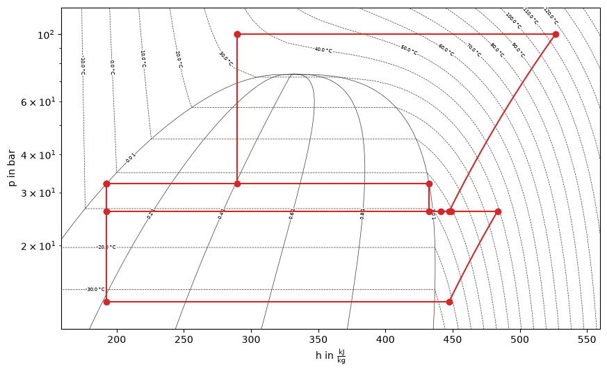
As a first guess, we operate the system at 100 bar. The COP drops sharply compared to the subcritical winter case, because of the higher heat rejection temperature and because almost half of the expanded mass flow turns into flash gas.

model.solve_model(
    gas_cooler_outlet_temperature_C=35, gas_cooler_pressure_bar=100
)

records["transcritical, 100 bar"] = model.get_results(indicators)
pd.Series(records["transcritical, 100 bar"], name="transcritical, 100 bar")

COP                          4.617918e+00
total_compressor_power_kW    5.528042e+01
hrhx_heat_kW                -1.552804e+02
flash_gas_fraction           4.045574e-01
discharge_temperature_C      1.154173e+02
gas_cooler_pressure_bar      1.000000e+02
receiver_pressure_bar        3.200000e+01
gas_cooler_discharge_kW     -3.249817e-10
Name: transcritical, 100 bar, dtype: float64

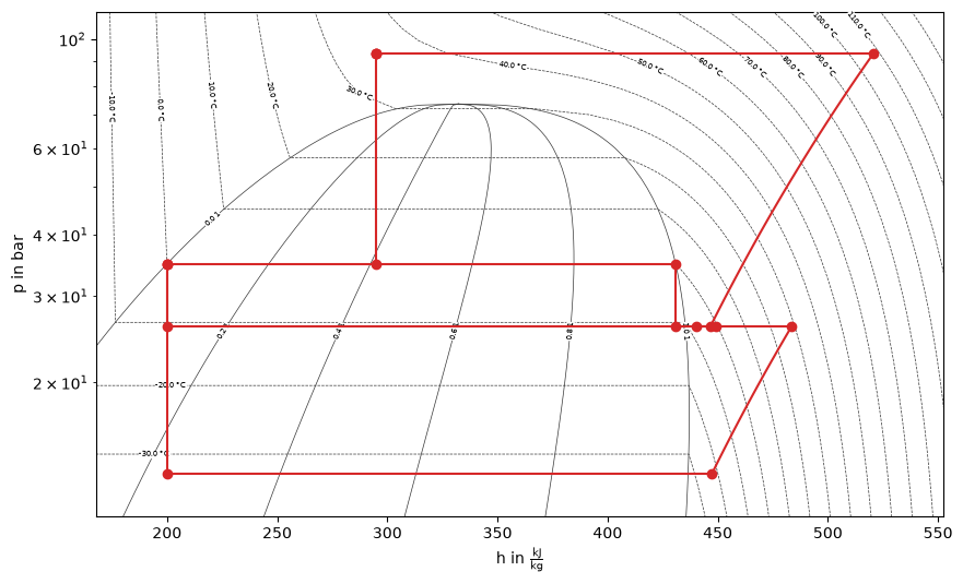
In the log(p)-h diagram we can see the process pressure going beyond the two phase dome.

fig, ax = model.plot_logph_diagram_matplotlib("c1")

The heat recovery heat exchanger now provides much more heat and at a higher temperature. The red line of the CO2 cooling down also shows the typical supercritical curvature of isobars in the TQ diagram.

fig, ax = model.plot_QT_diagram_matplotlib("heat-recovery-heat-exchanger")

Sensitivity: COP over gas cooler pressure

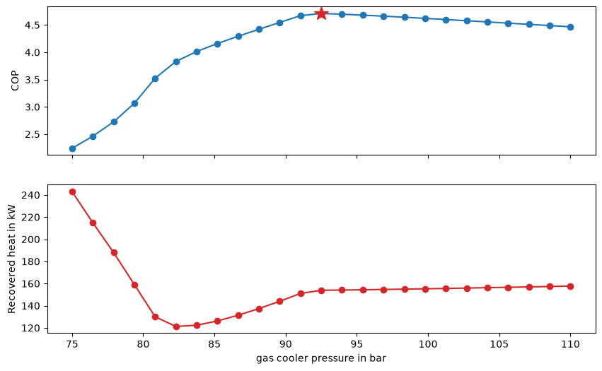
Before optimizing the cycle, a one dimensional parameter sweep visualizes the dependency between gas cooler pressure and COP. The sensitivity_analysis method of the base class runs one simulation per value, starting from the point closest to the current state and always stepping to the nearest unvisited point, which keeps the solver on a good initial guess throughout the sweep. The results are returned as a DataFrame in the requested order.

The COP curve shows the two competing effects: below roughly 85 bar the rising flash gas fraction dominates and the COP collapses, above 90 bar the additional compression work slowly reduces the efficiency. In between lies a distinct optimum. In the second row we plot the heat recovered.

sweep = model.sensitivity_analysis(
    param_dict={"gas_cooler_pressure_bar": np.linspace(75, 110, 25)},
    result_param_list=["COP", "flash_gas_fraction", "hrhx_heat_kW"],
)

fig, ax = plt.subplots(2, figsize=(10, 6), sharex=True)
ax[0].plot(sweep["gas_cooler_pressure_bar"], sweep["COP"], "o-", color="tab:blue")
sweep_best = sweep.loc[sweep["COP"].idxmax()]
ax[0].plot(
    sweep_best["gas_cooler_pressure_bar"], sweep_best["COP"],
    "*", color="tab:red", markersize=15
)
ax[0].set_ylabel("COP")
ax[1].plot(sweep["gas_cooler_pressure_bar"], -sweep["hrhx_heat_kW"], "o-", color="tab:red")
ax[1].set_ylabel("Recovered heat in kW")
ax[1].set_xlabel("gas cooler pressure in bar")
plt.close(fig)
fig

Optimization of the COP

The sweep only varied the gas cooler pressure. The receiver pressure is a second degree of freedom as it shifts the split between flash gas (throttled and recompressed by the MT compressor) and liquid supplied to the evaporators. The optimize method of the base class wraps pymoo and solves

\[\max_{p_\mathrm{gc},\; p_\mathrm{rec}} \quad \mathrm{COP}\left(p_\mathrm{gc}, p_\mathrm{rec}\right)\]

subject to the box bounds \(75 \leq p_\mathrm{gc} \leq 110\) bar and \(28 \leq p_\mathrm{rec} \leq 45\) bar. The lower receiver bound keeps a control margin above the MT evaporation pressure of 26 bar.

The decision variables and their bounds are regular parameter names from the lookup, so no extra glue code is needed. minimize_flags=[False] turns the minimization into a maximization, and the parameters passed as kpi are recorded alongside the objective for every evaluated individual. A particle swarm with 8 particles over 15 generations means 120 model evaluations.

Note

When this notebook is executed as part of a documentation build - locally or online - the number of generations is reduced to keep the build time short. Run the notebook interactively to execute the full 15 generations and reproduce the converged results discussed below.

n_gen = 15
if os.getenv("TESPY_DOCS_BUILD") or os.getenv("GITHUB_ACTIONS") == "true":
    n_gen = 2

log, result = model.optimize(
    algorithm=PSO(pop_size=8),
    termination=("n_gen", n_gen),
    variables={
        "gas_cooler_pressure_bar": {"min": 75, "max": 110},
        "receiver_pressure_bar": {"min": 28, "max": 45},
    },
    objective=["COP"],
    minimize_flags=[False],
    kpi=["flash_gas_fraction", "discharge_temperature_C", "hrhx_heat_kW"],
)

(
    log.sort_values("COP", ascending=False).head()
    .rename(columns={
        "gas_cooler_pressure_bar": "p gas cooler in bar",
        "receiver_pressure_bar": "p receiver in bar",
        "flash_gas_fraction": "flash gas fraction",
        "discharge_temperature_C": "T discharge in °C",
        "hrhx_heat_kW": "heat recovery in kW",
    })
    .style.format("{:.2f}")
    .format("{:.4f}", subset=["COP", "flash gas fraction"])
    .set_table_styles([{"selector": "th", "props": [("text-align", "left")]}])
    .set_properties(**{"text-align": "right"})
    .hide(axis="index")
)

p gas cooler in bar	p receiver in bar	COP	flash gas fraction	T discharge in °C	heat recovery in kW
93.31	34.89	4.6916	0.4117	107.76	-154.18
93.31	34.89	4.6916	0.4117	107.76	-154.18
92.23	38.54	4.6858	0.3963	106.02	-154.26
94.98	33.97	4.6774	0.4099	109.77	-154.39
90.73	30.57	4.6512	0.4478	105.18	-149.47

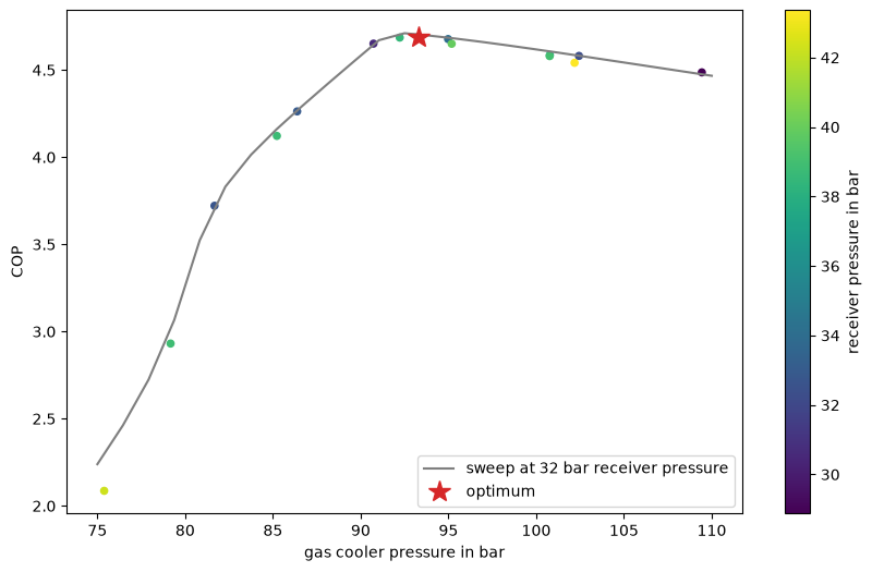
Plotting every evaluated individual on top of the sweep curve shows how the swarm converges towards the optimum. The color indicates the receiver pressure of each individual. Its influence on the COP is much weaker than that of the gas cooler pressure, so near the optimum the best individuals spread over a band of receiver pressures instead of collapsing onto a single value.

fig, ax = plt.subplots(figsize=(10, 6))
ax.plot(
    sweep["gas_cooler_pressure_bar"], sweep["COP"], "-", color="tab:gray",
    label="sweep at 32 bar receiver pressure"
)
sc = ax.scatter(
    log["gas_cooler_pressure_bar"], log["COP"],
    c=log["receiver_pressure_bar"], cmap="viridis", s=20
)
best = log.loc[log["COP"].idxmax()]
ax.plot(
    best["gas_cooler_pressure_bar"], best["COP"],
    "*", color="tab:red", markersize=15, label="optimum"
)
fig.colorbar(sc, label="receiver pressure in bar")
ax.set_xlabel("gas cooler pressure in bar")
ax.set_ylabel("COP")
ax.legend()
plt.close(fig)
fig

Best solution

To restore the optimal operating point, the best individual from the log is passed back through solve_model. The log(p)-h diagram of the optimized cycle shows the reduced high side pressure compared to the 100 bar run showed initially.

model.solve_model(
    gas_cooler_pressure_bar=best["gas_cooler_pressure_bar"],
    receiver_pressure_bar=best["receiver_pressure_bar"],
)

records["optimized"] = model.get_results(indicators)
fig, ax = model.plot_logph_diagram_matplotlib("c1")